Thermal emission spectra

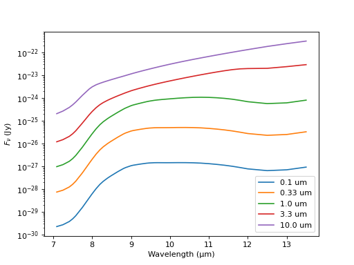
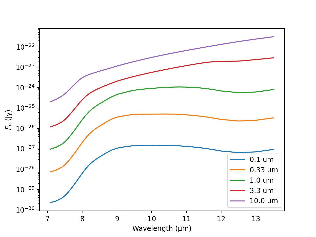
With the temperature of a grain calculated, its spectrum may be generated using the absorption efficiencies (\(Q_{abs}\)) and the Planck function. The following example calculates the spectrum of amorphous pyroxene grains from 0.1 to 10 μm (Mg/Fe=50/50) at 2 au from the Sun and 1 au from the observer, using the formula:

\[F_\nu = \frac{\pi a^2 Q_{abs} * B_{\nu}(T)}{\Delta^2}\]

First, setup our LTE instance. Note that here we are tracking units with astropy, but the LTE classes do not accept astropy quantities, so we use .value:

>>> import numpy as np
>>> import astropy.units as u
>>> from mskpy.util import planck
>>> from grains2 import PlaneParallelIsotropicLTE, ampyroxene50
>>>
>>> a = [0.1, 0.33, 1.0, 3.3, 10] * u.um
>>> ap50 = ampyroxene50()
>>> rh = 2.0 * u.au
>>> delta = 1.0 * u.au
>>>
>>> lte = PlaneParallelIsotropicLTE(a.value, ap50, rh.value)

\(Q_{abs}\) is a two-dimensional array. The first dimension is for grain size, the second dimension is for wavelength:

>>> lte.a.shape
(5,)
>>> lte.wave.shape
(322,)
>>> lte.Qabs.shape
(5, 322)

Now, calculate the spectra, limited to the 7 to 14 μm wavelength range:

>>> i = (lte.wave > 7) * (lte.wave < 14)
>>> wave = lte.wave[i]
>>> Qabs = lte.Qabs[:, i]
>>> F = np.zeros_like(Qabs) * u.Jy
>>> for i in range(len(lte.a)):
...     B = planck(lte.T[i], wave, unit="Jy/sr")
...     F[i] = (np.pi * a[i]**2 * Qabs[i] * B * u.sr / delta**2).to("Jy")

Plot the result:

(Source code, png, hires.png, pdf)