Grain size distributions

grains2 provides support for differential grain size distributions. For example, normal (Gaussian), Hansen modified gamma distribution, power-law, and the Hanner modified power-law functions are available.

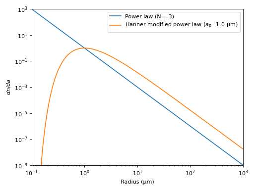
Create a power-law differential grain size distribution for grains from 0.1 μm to 1 mm with an index of –3:

>>> import numpy as np
>>> from grains2 import PowerLaw
>>>
>>> a = [0.1, 1.0, 1000]
>>> pl = PowerLaw(-3)
>>> pl.dnda(a)
array([1.e+03, 1.e+00, 1.e-09])

Compare this to a Hanner distribution with the same large particle slope (–3), but a peak grain size of 1.0 μm:

>>> from grains2 import Hanner
>>>
>>> h = Hanner(0.1, N=-3, ap=1.0)
>>> h.dnda(a)
array([0.00000000e+00, 1.00000000e+00, 5.83069613e+07])

Compare them in a plot:

(Source code, png, hires.png, pdf)